群馬大学 | 医学部 | サイトトップ | 医学情報処理演習
2009年12月24日
ある小学校の6年生は4クラスあり,職員室から近い順に,1組30人,2組28人,3組29人,4組30人が在籍している。ある週の月曜日,X先生は咳をしながら授業をしていたのだが,翌日高熱を発して欠勤し,近医を受診したところ,A型インフルエンザと診断された。水曜日,1組10人,2組5人,3組4人,4組1人がインフルエンザ様症状で学校を休んだため,1組は学級閉鎖になった(注:通常,校長が学級閉鎖を決定する目安は20%の欠席である。新型インフルエンザの場合,当初は1人でも患者が出たら全県が休校となったし,その後も暫くは10%の欠席で学級閉鎖とされていたが,現在では季節性インフルエンザと同様,20%になっている)。
この小学校6年生の4クラスにおいて,(1)欠席者の割合にはどのクラスでも差がないという帰無仮説を検定し,もし差があったなら,(2)どのクラスとどのクラスの間で差があるのかを検定せよ(検定の多重性はHolmの方法で調整すること)。また,(3)職員室から近いほどインフルエンザ罹患リスクが高く,リスクのスコアとして1組が4,2組が3,3組が2,4組が1であるという仮説が成り立つかどうか,コクラン=アーミテージ検定せよ。すべての検定に先立ち,クラスごとのインフルエンザ様疾患による欠席者割合を図示し,図と検定結果を参照して考察すること。
学籍番号・氏名とともに,下のフォームにRのコードと考察を貼り付けて送信せよ。
Consider 4 classes of 6th grade students in a primary school, where the numbers of pupils were 30, 28, 29, and 30 for the class 1, 2, 3, 4, respectively, and the class 1 is located nearest to the teachers' room. On Monday, one of the teachers, assuming his name as Mr. X, had classes with coughing. On Tuesday, high fever attacked Mr. X. Mr. X went to his home doctor, where he was diagnosed as type A influenza. On Wednesday, the numbers of absent pupils due to flu-like symptoms were 10, 5, 4, 1 for the class 1, 2, 3, 4, respectively. The class 1 was closed.
Answer the following questions. (1) Test the hypothesis that there is no difference among the absent proportions in these 4 classes. (2) If there is any difference, find the pairs with different absent proportion (Multiple comparison should be adjusted by Holm's method). (3) Assuming the risk to be dependent on the distance from the teachers' room, of which scores are 4, 3, 2, 1 for the classes 1, 2, 3, 4, respectively, test the null-hypothesis that there is no trend of the absent proportions dependent on this risk scores, using Cochran-Armitage test.
Write R scripts to do these hypothesis testing with appropriate graph drawings in the upper box. Discuss the results in the lower box. Never forget to write the student ID and name in each field.
Rのコードを次の枠内に示す。1行目〜3行目はデータをオブジェクトに付値し,名前を付けているだけである。4行目で4群間での割合の差の検定を行い,5行目で2群ずつの割合の差の検定を行い,holmの方法で第一種の過誤を調整している。このとき,期待度数が5未満のクラスがあるために,カイ二乗近似が不正確かもしれないという警告メッセージが表示されるので,本来は別解に示すようにフィッシャーの正確確率検定にすべきであり,また,2クラスずつの比較もフィッシャーの正確確率検定をHolmの方法で第一種の過誤を調整して実行すべきと思われるが,今回はそこまで要求しない。
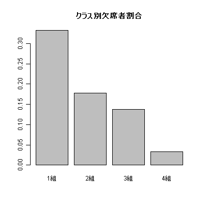
6行目では職員室からの距離に応じたリスクスコアを各クラスに割り当て,7行目でそれを使ってCochran-Armitageの検定を行っている。8行目ではクラス別欠席者割合を算出して棒グラフに表示させている。
pop <- c(30,28,29,30)
flu <- c(10,5,4,1)
names(pop) <- paste(1:4,"組",sep="")
prop.test(flu,pop)
pairwise.prop.test(flu,pop)
risk <- 4:1
prop.trend.test(flu,pop,risk)
barplot(flu/pop,main="クラス別欠席者割合")
結果は次の枠内の通りである。
    4-sample test for equality of proportions without continuity
    correction

data:  flu out of pop
X-squared = 9.8253, df = 3, p-value = 0.02011
alternative hypothesis: two.sided
sample estimates:
    prop 1     prop 2     prop 3     prop 4
0.33333333 0.17857143 0.13793103 0.03333333

    Pairwise comparisons using Pairwise comparison of proportions

data:  flu out of pop

  1     2     3
2 0.888 -     -
3 0.725 0.954 -
4 0.046 0.725 0.888

P value adjustment method: holm

    Chi-squared Test for Trend in Proportions

data:  flu out of pop ,
 using scores: 4 3 2 1
X-squared = 9.38, df = 1, p-value = 0.002194
検定の有意水準をいくつにするか,問題に示されていないので,通常の例にならい,以下すべての検定の有意水準を5%とする。
まず,prop.test()の結果,有意確率が0.02と有意水準以下なので,クラス間でインフルエンザ様疾患で休んだ子供の割合に有意な差があったといえる。Holmの方法で検定の多重性を調整した2クラスずつの比較の結果では(注:本来,Holmの方法による検定の多重性の調整は,有意水準の方を{1/k, 1/(k-1), ..., 1}倍したものと,ペアごとの検定の有意確率を小さい順に並べたものと比較するべきだが,Rの出力は有意確率が{k, k-1, ..., 1}倍されて表示されるので,常に有意水準である0.05と比較することで検定の有意性が判定できる),1組と4組の違いだけが統計学的に有意である。インフルエンザ様疾患で休んだ子供の割合(欠席者割合)がリスクスコアに対応した一定の傾向を示すことを対立仮説とするCochran-Armitage検定の結果,リスクスコアが高い(つまり職員室に近い)クラスほど欠席者割合が高い傾向が統計学的に有意であったことが示された。なお,図示は次の通り。
データの付値までは同様だが,それ以降をサンプルサイズが小さくても問題ない正確な検定に変えるのが,以下のコードである。
pop <- c(30,28,29,30)
flu <- c(10,5,4,1)
names(pop) <- paste(1:4,"組",sep="")
fisher.test(cbind(flu,pop-flu))

pairwise.fisher.test <- function(n1, n2) {
 if (length(n1)!=length(n2)) exit;
 nc <- length(n1)
 nnx <- ifelse(names(n2)!="",names(n2),as.character(1:nc))
 npairs <- sum(choose(nc,2))
 p.pairs <- numeric(npairs)
 x.pairs <- character(npairs)
 ni <- 0
 for (i in 1:(nc-1)) {
  for (j in (i+1):nc) {
   ni <- ni+1
   p.pairs[ni] <- fisher.test(matrix(c(n1[i],n1[j],n2[i]-n1[i],n2[j]-n1[j]),2,2))$p.value
   x.pairs[ni] <- paste(nnx[i],"-",nnx[j],sep="")
  }
 }
 names(p.pairs) <- x.pairs
 res <- sort(p.pairs)*npairs:1
 for (k in 1:npairs) { res[k] <- ifelse(res[k]>1,1,res[k]) }
 cat("** Exact pairwise comparison of proportions with **\n")
 cat("**       Holm's adjustment for multiplicity      **\n")
 print(data.frame(p.adj=res))
}

pairwise.fisher.test(flu,pop)
結果は以下のように得られる。Fisherの正確確率検定によっても,クラス間で統計学的に有意な欠席割合の差があり,Holmの方法で第一種の過誤を調整した2クラスずつの比較では,統計学的に有意な差が見られるのは1組と4組の間だけであり,カイ二乗近似をした場合と統計学的意思決定としては同じであった。
    Fisher's Exact Test for Count Data

data:  cbind(flu, pop - flu)
p-value = 0.01980
alternative hypothesis: two.sided

** Exact pairwise comparison of proportions with **
**       Holm's adjustment for multiplicity      **
             p.adj
1組-4組 0.03347455
2組-4組 0.48411122
1組-3組 0.50111361
3組-4組 0.58352932
1組-2組 0.47080405
2組-3組 0.72972614